Lecture 3 — Floating-Point Numbers in Computers
Handout: Foundations of and Exercises in Numerical Analysis
TipHow to use this handout — Evolving Study Notes with an AI Tutor
This handout is the main material for Lecture 3. The companion slides (3rd.html) only contain the exercise announcements and special class instructions; all the mathematical content lives here.
Like the Lecture 2 handout, this file is designed to grow with you. Whenever a line confuses you, ask the AI tutor (e.g. GitHub Copilot Chat in VS Code) and it will insert a Q&A block directly into this file, exactly where the question lives. Over the semester, your copy of this handout becomes your own annotated textbook.
The 30-second workflow
Step 0 — Once per chat session. Open AI_TUTOR.md in VS Code, then press ⌘L (Mac) / Ctrl+L (Win/Linux) so the file is attached to the chat, and send a short prime message such as:
Read this file. From now on, follow these rules whenever I ask
about my handout.
This gives the AI the Q&A format once, so you don’t have to re-attach it for every question.
Then, for each question:
- Open this handout (
3rd-handout.qmd) in the editor. - Select the line you don’t understand.
- Press
⌘L/Ctrl+L— your selection (and this file) are attached to the same chat as Step 0. - Just ask in plain language, e.g. “I don’t get this line — can you add a Q&A block here?”
- Re-render:
quarto render 3rd-handout.qmd— your question and its answer are now part of the handout (collapsed by default; click to expand).
💡 Why prime once with
AI_TUTOR.mdand then point with⌘L? The rules file is long; sending it every time wastes context. Loading it once and then pointing at the exact line you’re stuck on with⌘Lkeeps the AI focused on your question.
See AI_TUTOR.md at the repo root for the full rule set and the Q&A block format.
1 Recap from Lecture 2
In the previous lecture we saw that a real number can be expressed in the form
\[ \pm \left(\dfrac{d_0}{\beta^0} + \dfrac{d_1}{\beta^1} + \dfrac{d_2}{\beta^2} + \cdots\right)\cdot \beta^{e} \]
where
- \(\beta \geq 2\) is the base (e.g. 10, 2),
- each \(d_i\) is a digit with \(0 \leq d_i \leq \beta - 1\),
- \(e\) is an integer exponent.
Examples.
\[ 7.375 = + \left(\dfrac{7}{10^0} + \dfrac{3}{10^1} + \dfrac{7}{10^2} + \dfrac{5}{10^3}\right)\cdot 10^{0} \quad (\beta = 10) \]
\[ 7.375 = + \left(\dfrac{1}{2^0} + \dfrac{1}{2^1} + \dfrac{1}{2^2} + \dfrac{0}{2^3} + \dfrac{1}{2^4} + \dfrac{1}{2^5}\right)\cdot 2^{2} \quad (\beta = 2) \]
Some numbers are finite in one base but infinite in another:
\[ 0.2 = +\left(\dfrac{2}{10^0}\right)\cdot 10^{-1} \quad (\beta = 10) \quad\text{[finite]} \]
\[ 0.2 = +\left(\dfrac{1}{2^0} + \dfrac{1}{2^1} + \dfrac{0}{2^2} + \dfrac{0}{2^3} + \dfrac{1}{2^4} + \dfrac{1}{2^5} + \cdots\right)\cdot 2^{-3} \quad (\beta = 2) \quad\textbf{[infinite!]} \]
And \(\pi\) is infinite in both bases.
Today’s question. A computer cannot store infinitely many digits. So what does a number actually look like inside a computer?
2 Floating-Point Numbers in Computers
Since computers cannot hold infinitely many digits, they truncate the expansion above to a fixed length \(p\) and represent each number in the following finite form:
\[ \pm \left(\dfrac{d_0}{\beta^0} + \dfrac{d_1}{\beta^1} + \dfrac{d_2}{\beta^2} + \cdots + \dfrac{d_{p-1}}{\beta^{p-1}}\right)\cdot \beta^{e} \]
The block in parentheses is called the significand (sometimes mantissa). The format is fully described by four parameters:
| Symbol | Name | Meaning |
|---|---|---|
| \(\beta\) | base | Usually 2 (binary) on real computers |
| \(p\) | precision | Number of digits stored in the significand |
| \(e\) | exponent | Integer in a finite range \(E_{\min} \leq e \leq E_{\max}\) |
| \(d_i\) | digits | \(0 \leq d_i \leq \beta - 1\) |
NoteYour notes
(Why do you think computers chose \(\beta = 2\) instead of \(\beta = 10\)?)
3 IEEE 754 binary64 (a.k.a. double, float64)
Almost every modern CPU uses the IEEE 754 standard. Its 64-bit floating-point format — called binary64, double, or float64 — is the default for float in Python, double in C/Java, etc.
The 64 bits are laid out as:
| Field | Bits | What it stores |
|---|---|---|
| Sign | 1 bit | \(\pm\) |
| Exponent | 11 bits | \(e\) (with a bias of \(1023\)) |
| Significand | 52 bits | \(d_1, d_2, \ldots, d_{52}\) (the leading \(d_0\) is implicit) |
3.1 Why normalize? — to keep the representation unique
Looking back at the formula
\[ \pm \left(\dfrac{d_0}{2^0} + \dfrac{d_1}{2^1} + \cdots + \dfrac{d_{52}}{2^{52}}\right)\cdot 2^{e}, \]
if we put no restriction on \(d_0\), the same real number ends up having many different representations. For example, \(6 = (110)_2\) could be written as
\[ \begin{aligned} 6 &= (1.10)_2 \cdot 2^{2} \\ &= (0.110)_2 \cdot 2^{3} \\ &= (0.0110)_2 \cdot 2^{4} \\ &= (11.0)_2 \cdot 2^{1} \\ &= \cdots \end{aligned} \]
All of these correspond to the same value, just shifted by adjusting the exponent. This redundancy is bad for two reasons:
- Wasted precision. The leading zeros in \((0.0110)_2\) carry no information — they only push the meaningful bits further right and shrink the effective precision.
- Comparison/arithmetic gets hard. “Are these two bit patterns equal?” should be a simple bit check, not a non-trivial computation.
So the standard pins down a unique representation by requiring
\[ d_0 = 1. \]
Numbers that satisfy this are called normalized numbers. With this rule, \(6\) has exactly one representation: \((1.10)_2 \cdot 2^{2}\).
NoteBonus: the “hidden bit”
Because \(d_0\) is always \(1\) for normalized numbers, we don’t even need to store it. The 52 stored bits give us 53 bits of effective precision for free. This trick is built into IEEE 754 binary64.
3.1.1 The smallest positive normalized number
If we stick strictly with normalized numbers (i.e. \(d_0 = 1\) always), the smallest positive number we can write down keeps only the leading \(d_0 = 1\) and pushes the exponent to its minimum \(E_{\min} = -1022\):
\[ m_n = \left(\dfrac{1}{2^0} + \dfrac{0}{2^1} + \dfrac{0}{2^2} + \cdots + \dfrac{0}{2^{52}}\right)\cdot 2^{-1022} = 1 \cdot 2^{-1022} \approx 2.225 \times 10^{-308}. \]
3.2 Denormalized numbers — fill the gap by trading precision for range
If every number had to be normalized, then everything in the gap \((0, m_n)\) would simply have to be rounded to \(0\) — an abrupt cliff. That feels wasteful: we still have plenty of bit patterns left over (those with \(d_0 = 0\) and \(e = -1022\)) that aren’t being used for anything.
To use those leftover bit patterns, the standard allows a second class of numbers, only at the very bottom of the range:
- \(d_0 = 0\)
- exponent fixed at \(e = -1022\)
These are called denormalized (or subnormal) numbers. The trade-off is precision: with \(d_0 = 0\), the leading \(1\) of the significand has moved into \(d_1\), \(d_2\), \(\ldots\) — every leading zero costs one bit of precision. In return, we can keep representing numbers that get gradually closer and closer to \(0\), instead of falling off a cliff at \(m_n\).
3.2.1 The smallest positive number representable in binary64
By taking \(d_0 = 0\), only the very last bit \(d_{52} = 1\), and \(e = -1022\), we squeeze out the smallest positive number that binary64 can represent at all:
\[ m_d = \left(\dfrac{0}{2^0} + \dfrac{0}{2^1} + \cdots + \dfrac{0}{2^{51}} + \dfrac{1}{2^{52}}\right)\cdot 2^{-1022} = 2^{-52} \cdot 2^{-1022} = 2^{-1074} \approx 4.941 \times 10^{-324}. \]
So the smallest positive float64 value is not \(m_n\) — it is this much tinier denormalized number.
| Class | \(d_0\) | \(e\) | Precision |
|---|---|---|---|
| Normalized | \(1\) | \(-1022 \leq e \leq 1023\) | full 53 bits |
| Denormalized | \(0\) | \(e = -1022\) (fixed) | gradually less than 53 bits |
| Special: \(\pm 0\), \(\pm\infty\), NaN | — | — | — |
Note that uniqueness of representation is still preserved (every denormalized number has \(d_0 = 0\) and \(e = -1022\), so each bit pattern still corresponds to exactly one real value). In short, denormalized numbers smoothly fill the gap between \(0\) and \(m_n\) without breaking uniqueness, expanding the expressive power of float64.
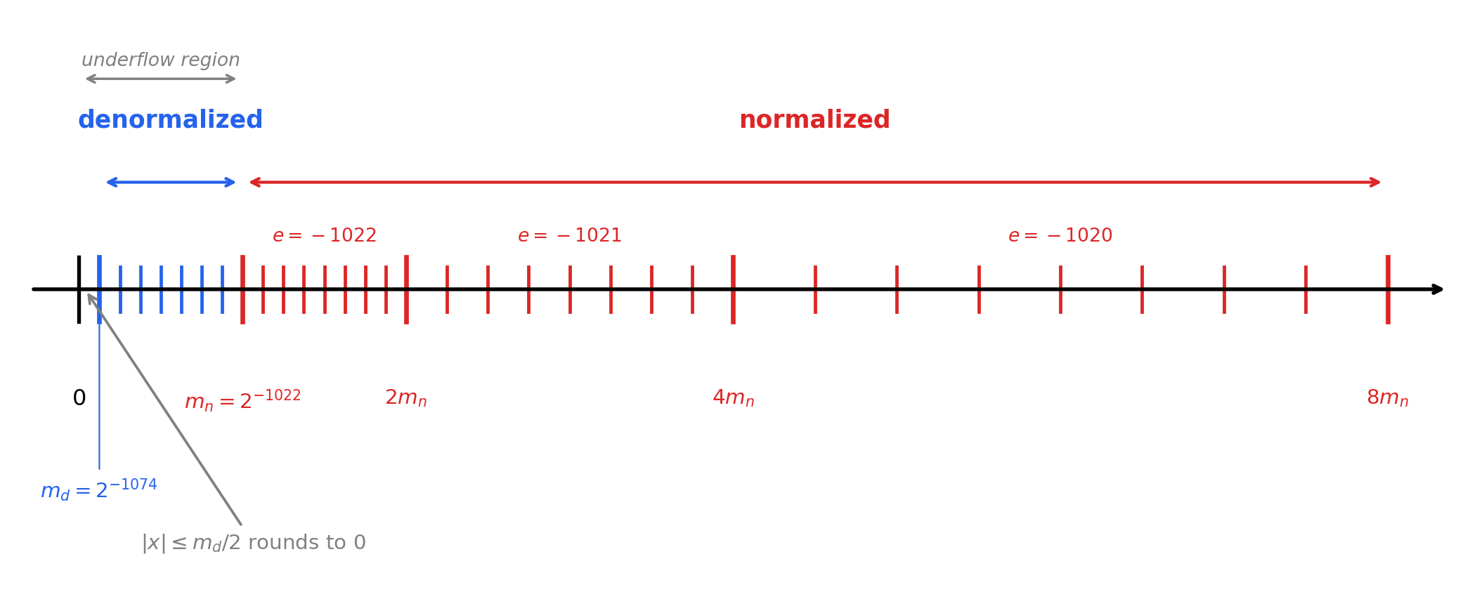
TipFloating-point numbers near \(0\) — a schematic picture
The schematic below shows how float64 numbers are scattered on the real line near zero. (The figure is generated by the Python code cell below — feel free to tweak it and re-render.)
What to notice:
- Normalized numbers (right, red): each band \(e = -1022, -1021, -1020, \ldots\) is twice as wide as the previous one, with the same number of equally-spaced ticks per band — so the spacing doubles with each step away from \(0\).
- Denormalized numbers (left, blue): all squeezed into the single band \(e = -1022\) with \(d_0 = 0\). The ticks are uniformly spaced at width \(2^{-1074} = m_d\).
- \(m_n = 2^{-1022}\) is the smallest normalized number; \(m_d = 2^{-1074}\) is the smallest positive
float64of any kind. - Underflow is the situation where the result of a computation has magnitude less than \(m_n\). It does not automatically mean the value becomes \(0\): in IEEE 754’s gradual underflow the value is represented as a denormalized number (with reduced precision). Under round-to-nearest, only values with \(|x| \leq m_d / 2\) are rounded to \(0\) — the equality case (\(|x| = m_d/2\)) is a tie that goes to \(0\) by ties-to-even (because the last bit of \(0\) is even, while the last bit of \(m_d\) is odd). Values in \((m_d/2,\ m_d)\) instead round up to \(m_d\), not down to \(0\).
4 Largest Representable Number
We already derived the two smallest positive numbers — \(m_n\) (Section 3) and \(m_d\) — while introducing normalized and denormalized numbers. The remaining piece is the largest one.
4.1 Largest positive normalized number
Take every digit to its maximum and the exponent to its maximum:
\[ M = \left(\dfrac{1}{2^0} + \dfrac{1}{2^1} + \cdots + \dfrac{1}{2^{52}}\right)\cdot 2^{1023} = (2 - 2^{-52})\cdot 2^{1023} \approx 1.798\times 10^{308}. \]
4.2 Summary — the three landmark values
Together, \(m_d\), \(m_n\), and \(M\) bracket the positive float64 range:
| Symbol | Value | Meaning |
|---|---|---|
| \(m_d\) | \(2^{-1074} \approx 4.941 \times 10^{-324}\) | smallest positive float64 (denormalized) |
| \(m_n\) | \(2^{-1022} \approx 2.225 \times 10^{-308}\) | smallest positive normalized float64 |
| \(M\) | \((2 - 2^{-52})\cdot 2^{1023} \approx 1.798 \times 10^{308}\) | largest positive float64 |
Real numbers far below \(m_d\) in magnitude round to \(0\) (underflow) and far above \(M\) become \(\pm\infty\) (overflow). But values just outside the range — slightly smaller than \(m_d\), or slightly larger than \(M\) — instead round inward to \(m_d\) or \(M\) respectively, since under round-to-nearest the closest representable float64 is the boundary itself.
NoteVerify in Python — what would this print?
import sys
fi = sys.float_info

# m_d = 2**-1074           (smallest positive float64, denormalized)
print(f"m_d  formula = 2**-1074                = {2.0**-1074:.6e}")
print()

# m_n = 2**-1022           (smallest positive normalized float64)
print(f"m_n  formula = 2**-1022                = {2.0**-1022:.6e}")
print(f"     Python  = sys.float_info.min      = {fi.min:.6e}")
print()

# M = (2 - 2**-52) * 2**1023  (largest positive float64)
print(f"M    formula = (2 - 2**-52) * 2**1023  = {(2 - 2**-52) * 2.0**1023:.6e}")
print(f"     Python  = sys.float_info.max      = {fi.max:.6e}")
Tip▶ Click to reveal the output
m_d  formula = 2**-1074                = 4.940656e-324

m_n  formula = 2**-1022                = 2.225074e-308
     Python  = sys.float_info.min      = 2.225074e-308

M    formula = (2 - 2**-52) * 2**1023  = 1.797693e+308
     Python  = sys.float_info.max      = 1.797693e+308
5 Rounding “Nearest”
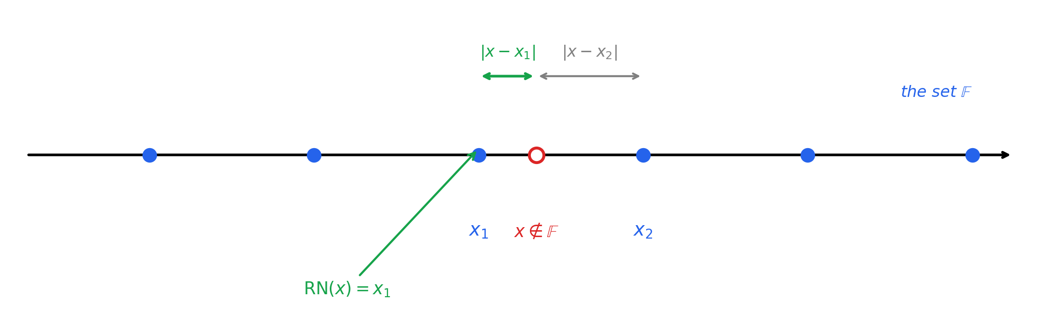
Most real numbers \(x \in \mathbb{R}\) are not exactly representable in binary64. So when a computer is asked to store \(x\), it has to round it to a representable number.
Let \(\mathbb{F}\) denote the set of all binary64 numbers, and pick a normalized \(x\) satisfying \(m_n \leq x \leq M\).
5.1 Other rounding modes
IEEE 754 actually defines four rounding modes. Round-to-nearest is the default and the one we use throughout the course.
| Mode | Symbol | Picks |
|---|---|---|
| Round to nearest (even) | \(\mathrm{RN}\) | closest in \(\mathbb{F}\); tie → even significand |
| Round toward \(+\infty\) | \(\mathrm{RU}\) | upward / ceiling in \(\mathbb{F}\) |
| Round toward \(-\infty\) | \(\mathrm{RD}\) | downward / floor in \(\mathbb{F}\) |
| Round toward zero | \(\mathrm{RZ}\) | truncation in \(\mathbb{F}\) |
We will revisit \(\mathrm{RU}\) and \(\mathrm{RD}\) in a later lecture on interval arithmetic.
5.2 Observation: rounding around \(1\)
Look at the gap between \(1\) and the next representable number larger than \(1\). Call this gap \(\varepsilon\).
By definition both \(1\) and \(1 + \varepsilon\) live in \(\mathbb{F}\), but their last stored bits are different:
\[ 1 \;=\; \Bigl(\tfrac{1}{2^0} + \tfrac{0}{2^1} + \tfrac{0}{2^2} + \cdots + \tfrac{\boldsymbol{0}}{2^{52}}\Bigr)\cdot 2^{0} \qquad (d_{52} = 0) \]
\[ 1 + \varepsilon \;=\; \Bigl(\tfrac{1}{2^0} + \tfrac{0}{2^1} + \cdots + \tfrac{0}{2^{51}} + \tfrac{\boldsymbol{1}}{2^{52}}\Bigr)\cdot 2^{0} \qquad (d_{52} = 1) \]
Now ask the computer to round three reals between them: \(1 + \tfrac{\varepsilon}{4}\), \(1 + \tfrac{\varepsilon}{2}\), and \(1 + \tfrac{3\varepsilon}{4}\). Where do they go?
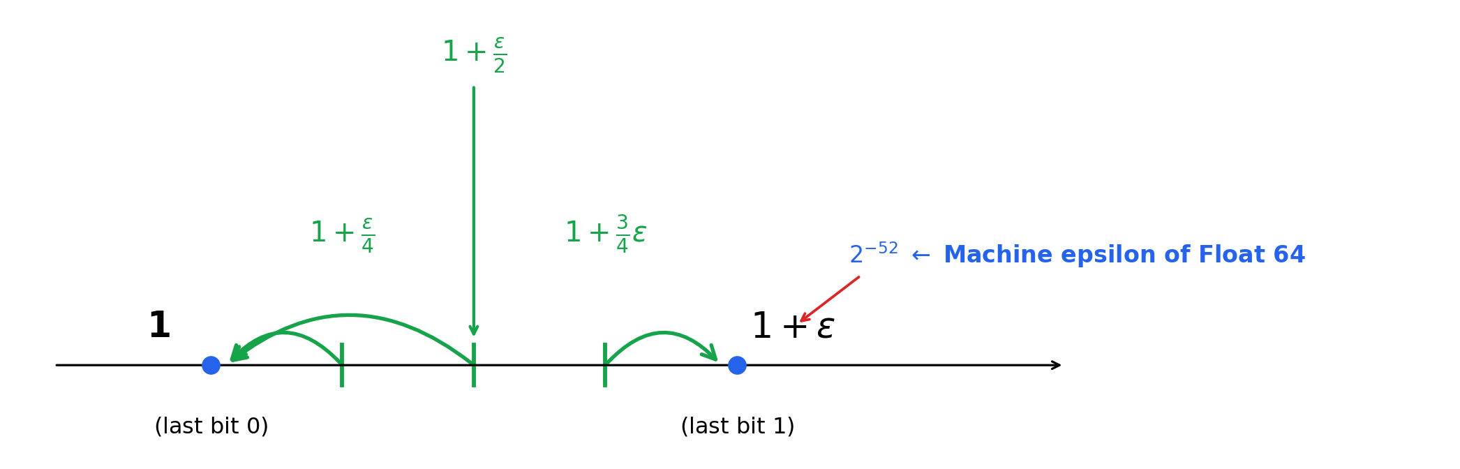
5.2.1 Machine epsilon
The gap we just used near \(1\) deserves a formal name. The machine epsilon of binary64 is
\[ \varepsilon \;:=\; 2^{-52} \;\approx\; 2.22\times 10^{-16}, \]
namely the distance from \(1\) to the next representable number in \(\mathbb{F}\). In Python it is also exposed as sys.float_info.epsilon.
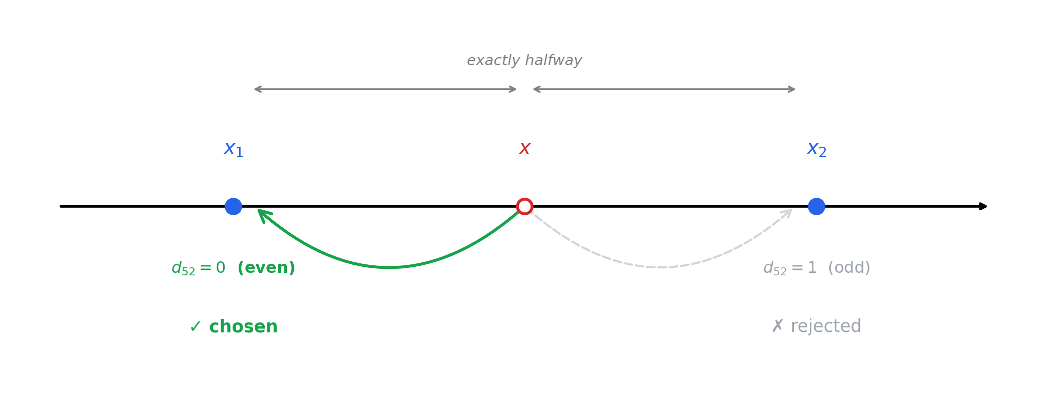
5.3 Special case: tie-breaking by “round to even”
When \(x\) falls exactly halfway between two representable numbers \(x_1\) and \(x_2\), round-to-nearest picks the one whose last stored digit is even (i.e. \(d_{52} = 0\)).
This rule keeps long sums of rounded values statistically unbiased — naive “always round up on ties” would consistently over-estimate.
NoteVerify in Python — the three values from above
eps = 2**-52   # = the gap between 1 and the next float64

print(f"(1 + ε/4)  - 1 = {(1 + eps/4)     - 1!r}")
print(f"(1 + ε/2)  - 1 = {(1 + eps/2)     - 1!r}")
print(f"(1 + 3ε/4) - 1 = {(1 + 3*eps/4)   - 1!r}")
Tip▶ Click to reveal the output
(1 + ε/4)  - 1 = 0.0
(1 + ε/2)  - 1 = 0.0
(1 + 3ε/4) - 1 = 2.220446049250313e-16
6 Summary
| Concept | Key fact |
|---|---|
| Floating-point format | \(\pm\) significand \(\cdot \beta^{e}\), with \(p\) digits in the significand |
| binary64 (IEEE 754) | \(\beta = 2\), \(p = 53\) effective bits (52 stored + 1 hidden), \(E_{\min} = -1022\), \(E_{\max} = 1023\) |
| Normalization | \(d_0 = 1\) ⇒ representation is unique and gains the hidden bit for free |
| Denormalized numbers | \(d_0 = 0\) at the smallest exponent — fill the gap near \(0\) by trading precision for range |
| Smallest positive denormalized | \(m_d = 2^{-1074} \approx 4.941 \times 10^{-324}\) |
| Smallest positive normalized | \(m_n = 2^{-1022} \approx 2.225 \times 10^{-308}\) |
| Largest positive | \(M = (2 - 2^{-52}) \cdot 2^{1023} \approx 1.798 \times 10^{308}\) |
| Machine epsilon | \(\varepsilon = 2^{-52} \approx 2.22 \times 10^{-16}\) — distance from \(1\) to the next float64 |
| Default rounding | Round to nearest (RN); on a tie, the side with even \(d_{52}\) wins |